
Enhanced XMM-Newton Spectral-fit Database
3XMM spectral-fit database (XMMFITCAT)
Contents
1. Automated spectral fitting
We used the fitting and modelling software Sherpa 4.9.1 (Freeman et al. 2001) to perform the automated spectral fits. We followed the Bayesian technique proposed in Buchner et al. (2014) using the analysis software BXA (Bayesian X-ray Analysis), which connects the nested sampling algorithm MultiNest (Feroz et al. 2013) with Sherpa.
In the BXA framework, the use of Cash fitting statistics is mandatory. We used the wstat implementation in Sherpa, which allows using background datasets as background models. To use this statistics, grouped spectra from the CATV catalogue were ungrouped, and then grouped to 1 count per bin.
All available instruments and exposures for a single observation of a source are fitted together. Only spectral data within the 0.5-10 keV band are fitted. All parameters for different instruments are tied together except for a relative normalization, which accounts for the differences between different flux calibrations.
1.1. Spectral data selection criteria
Spectral data from the CATV catalogue were screened before applying the automated spectral-fitting pipeline so that spectral fits are only performed if the data fulfil the following criteria:
- Only spectra corresponding to a single instrument and observation with more than 50 net counts (i.e. background subtracted) in the 0.5-10 keV band are used in the spectral fits. This means that some detections with more than 100 EPIC counts in the total band, but less than 50 counts in each different EPIC instrument, are excluded from the automated fits, and therefore, they are not included in the spectral-fit database.
- Complex models (see Sect.1.2), are only applied if the number of EPIC counts is larger than 500 net counts in the total band.
As a result of the application of these criteria, the spectral-fit database contains spectral-fitting results corresponding to the simple models in the full band for CATD source detections, corresponding to CATD unique sources. Spectral-fitting results for complex models are available for CATD source detections. The distribution of spectral counts per observation used during the automated fits is plotted in Fig. 1. Observations with more than 10,000 counts, 2% of the CATD detections, are excluded of this plot for clarity.
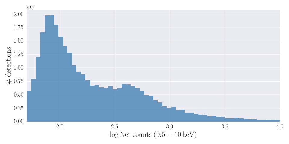 Figure 1. Distribution of net counts (background subtracted spectral counts) per observation used in the automated spectral fits. Observations with more than 10,000 counts are not included in this plot.
1.2. Spectral models
Most sources included in XMMPZCAT are extragalactic and hence the population is dominated by AGN. Given this fact, we have reduced the number of spectral models with respect to XMMFITCAT. They are phenomenological models selected to reproduced the spectral emission of AGN. We have also included a simple thermal model to deal with the X-ray emission of stars (about ten percent of XMMPZCAT sources) and other hot plasmas (e.g. intra-cluster medium emission).
There are four different models, two simple and two more complex models, as follows:
- Simple models:
- Absorbed power-law model (XSPEC: zwabs*pow): Variable parameters are the hydrogen column density of the absorber, the power-law photon index, and the power-law normalisation
- Absorbed thermal model (XSPEC: zwabs*mekal): Variable parameters are the hydrogen column density of the absorber, the plasma temperature of the thermal component, and the normalisation of the thermal component.
- Complex models:
- Absorbed thermal plus power-law model (XSPEC: zwabs*(mekal + zwabs*pow)): Variable parameters are the hydrogen column density of both absorbers, the plasma temperature, the photon index, and the normalisation of the power-law and thermal components.
- Absorbed double power-law model (XSPEC: zwabs*(pow + zwabs*pow)): Variable parameters are the hydrogen column density of both absorbers, the photon indices of both power-law components, and their normalisations.
All models include an additional wabs component to take into account the Galactic absorption, with its Hydrogen column density fixed to the value in the direction of the source from the Leiden/Argentine/Bonn (LAB) Survey of Galactic HI.
In the BXA framework we employed for the spectral fitting, a probability prior should be assigned to each free parameter in the model. These are the priors we selected:
- Hydrogen column density: Jeffreys prior (i.e. a uniform prior in the logarithmic space) with limits 1020 - 1025 cm-2.
- Power law photon index: gaussian prior with mean 1.9 and standard deviation 0.15. It corresponds to the photon index distribution for the AGN population as described in Nandra & Pounds, 1994.
- Thermal plasma temperature: uniform prior with limits 0.08 - 20 keV.
- Redshift: for sources with known spectroscopic redshift, this is included as a fixed parameter in the models. When only a photometric redshift is available, the redshift is treated as a free parameter using the photo-z probability density distribution given by MLZ/TPZ as the prior.
- Normalisation: Jeffreys prior with limits 10-30 - 1.
- Relative normalisation constants: Jeffreys prior with limits 0.01 - 100.
Examples of automated spectral fits for each of the spectral models used are plotted in Fig. 2. The photon index and NH distribution for detections for which an absorbed power-law model is an acceptable fit, >50% of the detections (see Sect.1.5), is shown in Fig. 3.
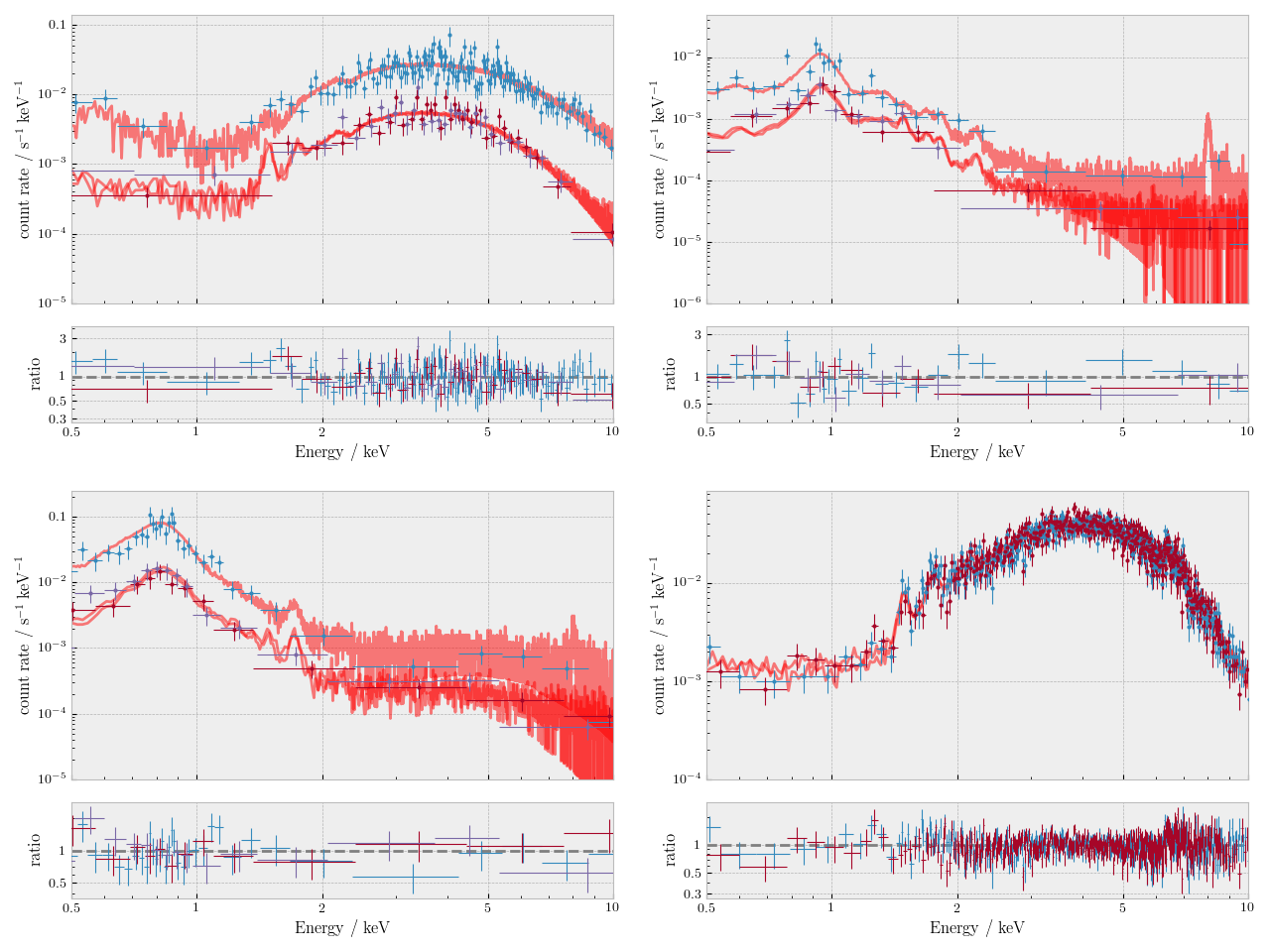 Figure 2. Examples of spectral fits for the four different models applied. Plots correspond to the unfolded (source+background) spectra and model over data to model ratio. From left to right and top to bottom: wabs*pow, wabs*mekal, wabs(mekal+wabs*pow), and wabs(pow+wabs*pow).
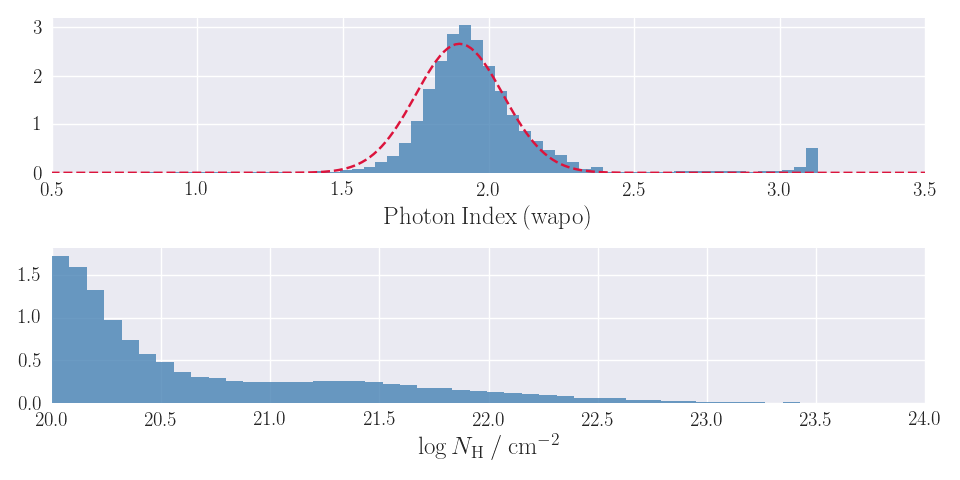 Figure 3. Photon index (top) and Hydrogen column density (bottom) distribution corresponding to the detections for which an absorbed power-law model in the full band is an acceptable fit. The dashed red line shows the selected prior for the photon index: a normal distribution with mean 1.9 and standard deviation 0.15.
1.3. Best-fit parameters and error computation
The MultiNest algorithm implemented in BXA gives the marginalized posterior probability distribution for all free parameters in the fitted model. We used these distributions to estimate the best-fit parameters and the corresponding errors. The best-fit values correspond to the mode (the most probable value) of the posterior distribution, estimated using a half-sample algorithm. Errors were estimated using the posterior distributions to calculate a 90% credible interval around the mode.
Figure 4 shows an example of the marginal and conditional (for two parameters) posterior distributions for a source fitted with a wabs*pow model. This example shows how the structure of the original photo-z probability distribution is preserved.
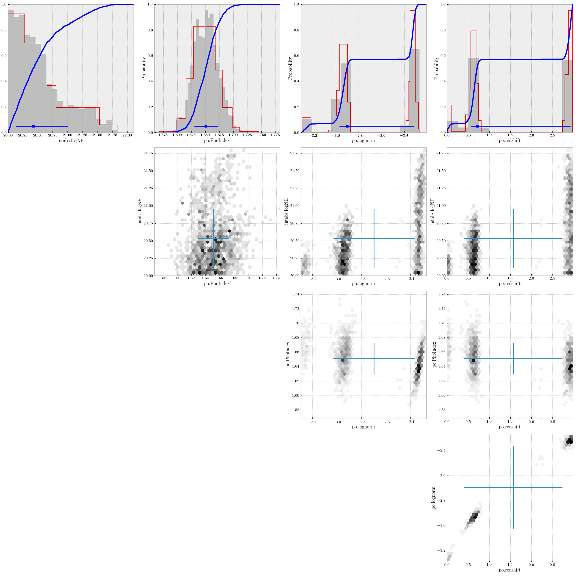 Figure 4. Example of posterior distributions for a source fitted with a wabs*pow model. Top row: marginal distributions. Remaining rows: two-parameter conditional distributions.
1.4. Goodness of fit
Cash maximum likelihood statistics lacks a direct estimate of goodness of fit (GoF). We followed the method proposed in Buchner et al. (2014) and we used Q-Q (quantile-quantile) plots to obtain an estimate of the GoF of our spectral fits.
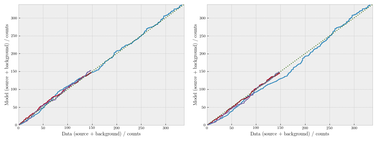 Figure 5. Q-Q plots for a source fitted with a zwabs*pow model (left) and a zwabs*mekal model (right). Blue, red and purple lines corresponds to PN, MOS1 and MOS2 data, respectively.
A Q-Q plot compares the cumulative counts of the data (source+background) with the predicted counts (source+background) of the model (see Figure 5 below). The plot gives a quick visual idea of how well the model can reproduce the data. For a quantitative estimate of the GoF we calculated the Kolmogorov-Smirnov (KS) statistic between the two cumulative distributions and the corresponding p-value. A low KS (or a high p-value) means that the data is well reproduced by the model.
Note however that in our case the p-values for these statistics cannot be calculated the usual way. The cumulative distribution of the model depends on the parameters that were estimated from the data distribution, therefore the condition of independence between the two compared distribution does not hold, and hence the probabilities estimated using the KS probability distribution are grossly incorrect. Nevertheles, through a permutation test we can get an estimate of the p-value. For each source, we did 1000 resamplings, randomly splitting the original data+model sample in two equal-size subsamples, and estimate the corresponding KS statistic. Our estimated p-values are the ratio of resamplings that have statistics larger than the statistic of the original samples.
Note also that the KS test is more sensitive for distributions with large counts. Therefore, for detections with more than 500 counts in the total band, a fit with KS p-value > 0.9 is considered acceptable. Otherwise, a p-value > 0.5 is considered an acceptable fit. Taking into account all the spectral models implemented in this database, an acceptable fit is found for about 90% of all the detections. Figure 6 shows the KS p-value distribution of the WAPO model.
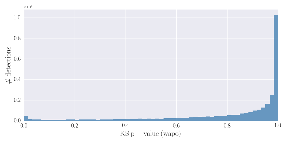 Figure 6. KS p-value distribution of the wabs*pow model.
2. Description of the columns
The XMMFITCAT-Z table contains one row for each detection, and 157 columns containing information about the source detection and the spectral-fitting results. Not available values are represented by an empty "NULL" value. The first 14 columns contain information about the source and observation, including redshift information, whereas the remaining 143 columns contain, for each model applied, model spectral-fit flags, parameter values and errors, fluxes, luminosities and five columns to describe the goodness of the fit.
2.1 Source and observation
IAUNAME: The IAU name assigned to an unique source in the CATV catalogue.
SC_RA, SC_DEC: Right ascension and declination in degrees (J2000) of the unique source, as in the CATV catalogue. RA and DEC correspond to the SC_RA and SC_DEC columns in the CATV catalogue. These are corrected source coordinates and, in the case of multiple detections of the same source, they correspond to the weighted mean of the coordinates for the individual detections.
SRCID: A unique number assigned to a group of catalogue entries which are assumed to be the same source in CATV.
DETID: A consecutive number which identifies each entry (detection) in the CATV catalogue.
OBS_ID: The XMM-Newton observation identification, as in CATV.
SRC_NUM: The (decimal) source number in the individual source list for this observation (OBS_ID), as in CATV. Note that in the pipeline products this number is used in hexadecimal form.
PHOT_Z, PHOT_ZERR: Photometric redshift of the source (from XMMPZCAT) and the corresponding 1σ error.
SPEC_Z: Spectroscopic redshift of the source, if available.
T_COUNTS/H_COUNTS/S_COUNTS: spectral background subtracted counts in the full/hard/soft bands computed by adding all available instruments and exposures for the corresponding observation.
GNH: Galactic column density in the direction of the source from the Leiden/Argentine/Bonn (LAB) Survey of Galactic HI.
2.2 Model related columns
Columns referring to any particular model start with the model's name. Model names are:
wapo: absorbed power-law model applied in the 0.5-10 keV band.
wamekal: absorbed thermal model applied in the 0.5-10 keV band.
wamekalpo: absorbed thermal plus power-law model applied in the 0.5-10 keV band.
wapopo: absorbed double power-law model applied in the 0.5-10 keV band.
2.2.1 Spectral-fit summary columns
The first three columns after the columns related to the source and observation, are A_FIT, P_MODEL, and A_MODELS.
A_FIT: The value is set to True, if an acceptable fit, i.e. KS p-value > 0.01, has been found for at least one of the models applied, and to False otherwise.
P_MODEL: The data preferred model, i.e., the model with the highest evidence (lowest logZ, see Sect. 2.2.4). A spectral model is always listed regardless of the fit being an acceptable or an unacceptable fit.
A_MODELS: List of acceptable models. This column contains the remaining models with relative evidence (with respect to P_MODEL) higher than 30 ('very strong evidence' accordingly to the scale of Jeffreys 1961). Assuming all models a priori equally probable, there is no statistical reason to rule out any of the models in the set formed by P_MODEL and A_MODELS. Hence, if the fit is acceptable, the simplex model should be selected as the best-fit model.
2.2.2 Parameters and errors
Columns referring to parameters and errors start with the model name and the parameter name. Possible parameters names are: logNH (decimal logarithm of wabs column density, in units of cm-2), PhoIndex (pow photon index), kT (mekal temperature, in keV), and z (redshift of the source, only for sources with no spectroscopic redshift). Values for the normalizations of the models and the relative normalization factors between instruments are not included in the table (but they are available in the SQL database).
MODEL_PARAMETER: parameter value.
MODEL_PARAMETER_min, MODEL_PARAMETER_max: upper and lower limits of the 90% credible interval for the parameter.
2.2.3 Fluxes and luminosities
The posterior probability distribution of the free parameters was propagated to estimate the flux and errors for each model. This method preserves the structure of the uncertainty (degeneracies, multimodal structure, etc.). Reported fluxes and luminosities in the catalogue correspond to the mode of the posterior distribution, with errors estimated as 90% credible intervals. These are EPIC fluxes, i.e., in the case of multiple instrument spectra for a single observation, the reported flux is the average of the different fluxes for each instrument and exposure.
For sources with spectroscopic redshifts, luminosities were estimated using the intrinsic fluxes and the luminosity distance corresponding to that redshift. For sources with photometric redshifts, z is a free parameter and hence is propagated with the posterior distribution to estimate the corresponding luminosity distance in each case. We assumed a ΛCDM cosmology with H0 = 67.7, Ωm = 0.307 (Planck Collaboration 2015, Paper XIII).
We estimated fluxes and luminosities in the soft (0.5-2 keV) and hard (2-10 keV) bands. For observed fluxes this bands correspond to the observer frame. For intrinsic fluxes and luminosities they correspond to the source's rest frame.
EPIC soft fluxes obtained from the spectral fits (P_MODEL) are plotted against the ones in the CATV catalogue (EP_2_FLUX + EP_3_FLUX) in Fig. 7. Fluxes from the automated fits and from the CATV are consistent within errors for ∼70% of the detections. Significant differences between both values are more frequent among sources displaying a soft spectrum, i.e., those sources that are best-fitted by a power-law with a steep photon index, or by a thermal model. More than 80% of the non-matching fluxes correspond to any of these cases. Figure 8 shows hard luminosities against redshifts estimated in the automated fits for P_MODEL.
MODEL_flux_BAND: the mean observed flux (in erg cm-2 s-1) of all instruments and exposures for the corresponding observation, in "BAND" (soft/hard). Observed fluxes were corrected of Galactic absorption.
MODEL_fluxmin_BAND, MODEL_fluxmax_BAND: lower and upper limits of the 90% credible interval.
MODEL_intflux_BAND: the mean intrinsic flux (rest-frame, corrected of intrinsic absorption, in erg cm-2 s-1) of all instruments and exposures for the corresponding observation, in "BAND" (soft/hard).
MODEL_intfluxmin_BAND, MODEL_intfluxmax_BAND: lower and upper limits of the 90% credible interval.
MODEL_lumin_BAND: the mean luminosity (rest-frame, corrected of intrinsic absorption, in erg s-1) of all instruments and exposures for the corresponding observation, in "BAND" (soft/hard).
MODEL_luminmin_BAND, MODEL_luminmax_BAND: lower and upper limits of the 90% credible interval.
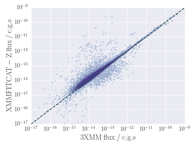 Figure 7. Soft fluxes (in c.g.s. units) computed from the automated fits (P_MODEL) against fluxes in the CATV catalogue.
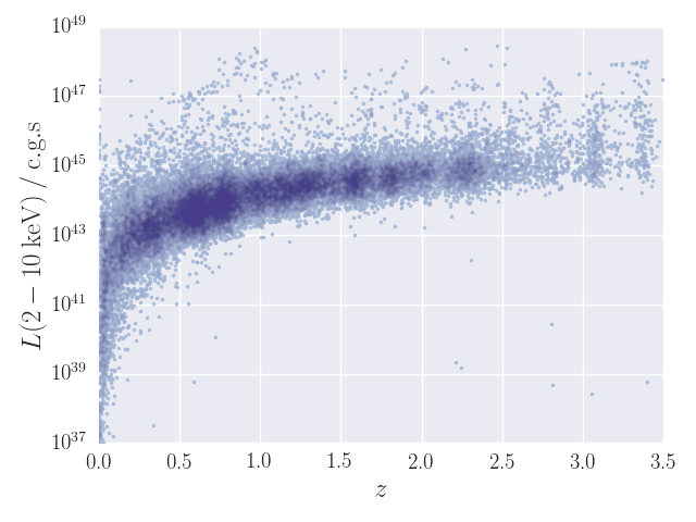 Figure 8. Hard luminosity versus redshift (in c.g.s. units) computed from the automated fits (P_MODEL).
2.2.4 Fitting statistics
MODEL_wstat: W-stat (Cash statistics) value.
MODEL_dof: Degrees of freedom.
MODEL_ks: Kolmogorov-Smirnov (KS) statistic.
MODEL_ks_pvalue: KS p-value.
MODEL_logZ: Natural logarithm of the evidence, estimated by the MultiNest algorithm.
© Copyright IAASARS/NOA | Courtesy of Open Web Design | A. Ruiz, webmaster